
주제 : 이미지를 100%의 정확도로 구분하는 모델 만들기
**추가----------------------------------
혹시 블로그에 사용한 이미지데이터가 필요하신 분은 아래 댓글이나 이메일 보내주시면 그냥 보내드립니다~
질문은 메일보다 댓글로 적어주세요!!
연락주실 때 블로그 아래 하트모양 공감 꼭 눌러주세요
(혹시 메일이 안오면 공감 눌렀는지 확인하세요!!)
전부 했는데도 안오면 아래 메일로 데이터 요청해주시면 좀 더 빠른 답장 드릴게요
E-mail : rnjswodn2443@naver.com
-----------------------------------------

데이터
- 총 이미지 : 13798개
- 라벨 : 8개
- person(1972개)
- airplane(1454개)
- car(1936개)
- dog(1404개)
- cat(1770개)
- flower(1686개)
- fruit(2000개)
- motorbike(1576개)
데이터 구조
imagedata
└ person
└ airplane
└ car
└ dog
└ cat
└ flower
└ fruit
└ motorbike
목표
- 분류 모델 성능 : 100 % 달성
작업 순서
- 데이터 불러오기
- 이미지 전처리
- 베이스라인 모델 설정
- 모델 튜닝 후 성능 높이기
- 데이터 증강
- 전이 학습
- 모델 성능 확인
- 결론
import os.path
import cv2
import numpy as np
import pandas as pd
import matplotlib.pyplot as plt
import tensorflow as tf
import seaborn as sns

from pathlib import Path
from tqdm import tqdm
from time import perf_counter

from sklearn.model_selection import train_test_split
from sklearn.metrics import classification_report,accuracy_score
from IPython.display import Markdown, display
데이터 불러오기(드라이브 마운트)
from google.colab import drive
drive.mount('/content/drive')
이미지 경로를 데이터 프레임 형태로 만드는 함수
dir_ = Path('/content/drive/MyDrive/Colab Notebooks/Data_analysis_Project/03_딥러닝_이미지분류/imagedata')
filepaths = list(dir_.glob(r'**/*.jpg'))
def proc_img(filepath):
    """
   		이미지데이터의 경로와 label데이터로 데이터프레임 만들기
    """

    labels = [str(filepath[i]).split("/")[-2] \
              for i in range(len(filepath))]

    filepath = pd.Series(filepath, name='Filepath').astype(str)
    labels = pd.Series(labels, name='Label')

    # 경로와 라벨 concatenate
    df = pd.concat([filepath, labels], axis=1)

    # index 재설정
    df = df.sample(frac=1,random_state=0).reset_index(drop = True)

    return df

df = proc_img(filepaths)
df.head(5)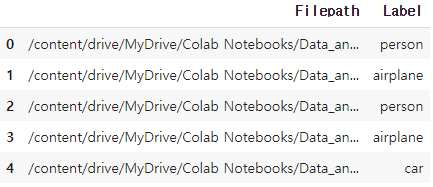
print(f'Number of pictures: {df.shape[0]}\n')
print(f'Number of different labels: {len(df.Label.unique())}\n')
print(f'Labels: {df.Label.unique()}')
Number of pictures: 13798
Number of different labels: 8
Labels: ['person' 'airplane' 'car' 'dog' 'cat' 'flower' 'fruit' 'motorbike']
- 이미지 데이터 확인
# 데이터 확인
fig, axes = plt.subplots(nrows=4, ncols=10, figsize=(15, 7),
                        subplot_kw={'xticks': [], 'yticks': []})

for i, ax in enumerate(axes.flat):
    ax.imshow(plt.imread(df.Filepath[i]))
    ax.set_title(df.Label[i], fontsize = 12)
plt.tight_layout(pad=0.5)
plt.show()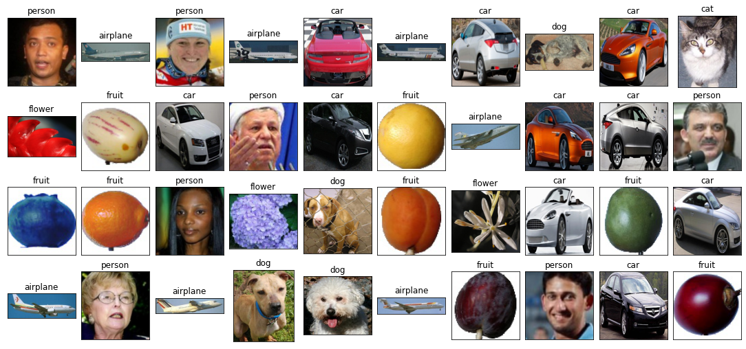
Label Category 분포 확인
vc = df['Label'].value_counts()
plt.figure(figsize=(9,5))
sns.barplot(x = vc.index, y = vc, palette = "rocket")
plt.title("Number of pictures of each category", fontsize = 15)
plt.show()
이미지 데이터 Train, Test 데이터로 분류
# Training/test split
# train_df,test_df = train_test_split(df.sample(frac=0.2), test_size=0.1,random_state=0) #모델링 시간이 오래걸리면 사용
train_df,test_df = train_test_split(df, test_size=0.1,random_state=0)
train_df.shape,test_df.shape
((12418, 2), (1380, 2))
베이스 라인 모델
모델 전처리
import numpy as np
import tensorflow as tf


from keras.preprocessing.image import ImageDataGenerator

train_datagen = ImageDataGenerator(rescale = 1./255,
                                   validation_split=0.2)

train_gen = train_datagen.flow_from_directory('/content/drive/MyDrive/Colab Notebooks/Data_analysis_Project/03_딥러닝_이미지분류/imagedata/data/natural_images',
                                                 target_size = (150, 150),
                                                 batch_size = 32,
                                                 class_mode = 'categorical',subset='training')
val_gen  = train_datagen.flow_from_directory('/content/drive/MyDrive/Colab Notebooks/Data_analysis_Project/03_딥러닝_이미지분류/imagedata/data/natural_images',
                                                 target_size = (150, 150),
                                                 batch_size = 32,
                                                 class_mode = 'categorical',subset='validation')
Found 5522 images belonging to 8 classes.
Found 1377 images belonging to 8 classes.
딥러닝 CNN모델로 베이스라인 모델링
# Initialising the CNN
cnn = tf.keras.models.Sequential()

# Step 1 - Convolution
cnn.add(tf.keras.layers.Conv2D(filters=32, kernel_size=3, activation='relu', input_shape=[150, 150, 3]))

# Step 2 - Pooling
cnn.add(tf.keras.layers.MaxPool2D(pool_size=2, strides=2))

# Adding convolutional layer
cnn.add(tf.keras.layers.Conv2D(filters=32, kernel_size=3, activation='relu'))
cnn.add(tf.keras.layers.MaxPool2D(pool_size=2, strides=2))

# Step 3 - Flattening
cnn.add(tf.keras.layers.Flatten())

# Step 4 - Full Connection
cnn.add(tf.keras.layers.Dense(units=128, activation='relu'))

# Step 5 - Output Layer
cnn.add(tf.keras.layers.Dense(units=8, activation='softmax'))

# Compiling the CNN
cnn.compile(optimizer = 'adam',
            loss = 'categorical_crossentropy',
            metrics = ['accuracy'])
cnn.summary()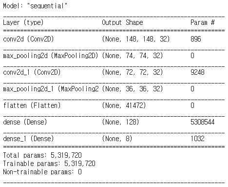
모델 성능 확인(accuracy)
cnn.fit(x = train_gen, validation_data = val_gen, epochs = 10)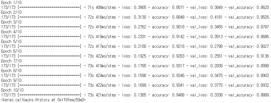
- 베이스 라인 모델 성능 결과
- accuracy : 0.9488
- val_accuracy : 0.8932
간단한 전처리 후 성능을 확인했는데 생각보다 높은 성능을 나타내서 조금 놀랬다.
하지만 나의 목표는 100%의 성능을 나타내는 모델을 만드는 것이기 때문에 모델의 성능을 높이는 작업을 해보겠다.
모델 성능 높이기
데이터 증강(Data Augmentation)으로 이미지 로드
def create_gen():
    # 생성기 및 데이터 증강으로 이미지 로드
    train_generator = tf.keras.preprocessing.image.ImageDataGenerator(
        preprocessing_function=tf.keras.applications.mobilenet_v2.preprocess_input,
        validation_split=0.1
    )

    test_generator = tf.keras.preprocessing.image.ImageDataGenerator(
        preprocessing_function=tf.keras.applications.mobilenet_v2.preprocess_input
    )

    train_images = train_generator.flow_from_dataframe(
        dataframe=train_df,
        x_col='Filepath', # 파일위치 열이름
        y_col='Label', # 클래스 열이름
        target_size=(224, 224), # 이미지 사이즈
        color_mode='rgb', # 이미지 채널수
        class_mode='categorical', # Y값(Label값)
        batch_size=32,
        shuffle=True, # 데이터를 섞을지 여부
        seed=0,
        subset='training', # train 인지 val인지 설정
        rotation_range=30, # 회전제한 각도 30도
        zoom_range=0.15, # 확대 축소 15%
        width_shift_range=0.2, # 좌우이동 20%
        height_shift_range=0.2, # 상하이동 20%
        shear_range=0.15, # 반시계방햐의 각도
        horizontal_flip=True, # 좌우 반전 True
        fill_mode="nearest"
        # 이미지 변경시 보완 방법 (constant, nearest, reflect, wrap) 4개 존재
    )

    val_images = train_generator.flow_from_dataframe(
        dataframe=train_df,
        x_col='Filepath',
        y_col='Label',
        target_size=(224, 224),
        color_mode='rgb',
        class_mode='categorical',
        batch_size=32,
        shuffle=True,
        seed=0,
        subset='validation',
        rotation_range=30,
        zoom_range=0.15,
        width_shift_range=0.2,
        height_shift_range=0.2,
        shear_range=0.15,
        horizontal_flip=True,
        fill_mode="nearest"
    )

    test_images = test_generator.flow_from_dataframe(
        dataframe=test_df,
        x_col='Filepath',
        y_col='Label',
        target_size=(224, 224),
        color_mode='rgb',
        class_mode='categorical',
        batch_size=32,
        shuffle=False
    )

    return train_generator,test_generator,train_images,val_images,test_images
회전각도, 확대축소, 좌우이동, 상하이동, 좌우반전 등 데이터 증강의 많은 기법을 사용해서 Train과 Val 데이터에 적용했고 Test 데이터는 학습에 사용되지 않기 때문에 증강기법을 적용하지 않았다.
전이학습을 사용해서 모델 성능 높이기
models = {
    "DenseNet121": {"model":tf.keras.applications.DenseNet121, "perf":0},
    "MobileNetV2": {"model":tf.keras.applications.MobileNetV2, "perf":0},
    "DenseNet201": {"model":tf.keras.applications.DenseNet201, "perf":0},
    "EfficientNetB0": {"model":tf.keras.applications.EfficientNetB0, "perf":0},
    "EfficientNetB1": {"model":tf.keras.applications.EfficientNetB1, "perf":0},
    "InceptionV3": {"model":tf.keras.applications.InceptionV3, "perf":0},
    "MobileNetV2": {"model":tf.keras.applications.MobileNetV2, "perf":0},
    "MobileNetV3Large": {"model":tf.keras.applications.MobileNetV3Large, "perf":0},
    "ResNet152V2": {"model":tf.keras.applications.ResNet152V2, "perf":0},
    "ResNet50": {"model":tf.keras.applications.ResNet50, "perf":0},
    "ResNet50V2": {"model":tf.keras.applications.ResNet50V2, "perf":0},
    "VGG19": {"model":tf.keras.applications.VGG19, "perf":0},
    "VGG16": {"model":tf.keras.applications.VGG16, "perf":0},
    "Xception": {"model":tf.keras.applications.Xception, "perf":0}
}
# Create the generators
train_generator,test_generator,train_images,val_images,test_images=create_gen()
print('\n')

def get_model(model):
# Load the pretained model
    kwargs =    {'input_shape':(224, 224, 3),
                'include_top':False,
                'weights':'imagenet',
                'pooling':'avg'}

    pretrained_model = model(**kwargs)
    pretrained_model.trainable = False # 레이어를 동결 시켜서 훈련중 손실을 최소화 한다.

    inputs = pretrained_model.input

    x = tf.keras.layers.Dense(128, activation='relu')(pretrained_model.output)
    x = tf.keras.layers.Dense(128, activation='relu')(x)

    outputs = tf.keras.layers.Dense(8, activation='softmax')(x)
    # 라벨 개수가 8개이기 때문에 Dencs도 8로 설정
    model = tf.keras.Model(inputs=inputs, outputs=outputs)

    model.compile(
        optimizer='adam',
        loss='categorical_crossentropy',
        metrics=['accuracy']
    )

    return model

# Train모델 학습
for name, model in models.items():

    # 전이 학습 모델 가져오기
    m = get_model(model['model'])
    models[name]['model'] = m

    start = perf_counter()

    # 모델 학습
    history = m.fit(train_images,validation_data=val_images,epochs=1,verbose=0)

    # 학습시간과 val_accuracy 저장
    duration = perf_counter() - start
    duration = round(duration,2)
    models[name]['perf'] = duration
    print(f"{name:20} trained in {duration} sec")

    val_acc = history.history['val_accuracy']
    models[name]['val_acc'] = [round(v,4) for v in val_acc]
다음으로는 전이학습 모델을 가지고와서 학습에 사용했는데 어떤 전이학습이 좋은 효율을 나타내는지 모르기 떄문에 전이학습 모델들을 전부가지고 와서 비교해보는 코드를 작성했다. 만들어 놓은 모델 함수에 for반복문을 통해서 전이학습모델을 전부 학습했다.
Test 데이터로 성능 확인
# test데이터로 모델 성능 예측
for name, model in models.items():

    # Predict the label of the test_images
    pred = models[name]['model'].predict(test_images)
    pred = np.argmax(pred,axis=1)

    # Map the label
    labels = (train_images.class_indices)
    labels = dict((v,k) for k,v in labels.items())
    pred = [labels[k] for k in pred]

    y_test = list(test_df.Label)
    acc = accuracy_score(y_test,pred)
    models[name]['acc'] = round(acc,4)
    print(f'**{name} has a {acc * 100:.2f}% accuracy on the test set**')

# Create a DataFrame with the results
models_result = []

for name, v in models.items():
    models_result.append([ name, models[name]['val_acc'][-1],
                          models[name]['acc'],
                          models[name]['perf']])

df_results = pd.DataFrame(models_result,
                          columns = ['model','val_accuracy','accuracy','Training time (sec)'])
df_results.sort_values(by='accuracy', ascending=False, inplace=True)
df_results.reset_index(inplace=True,drop=True)
df_results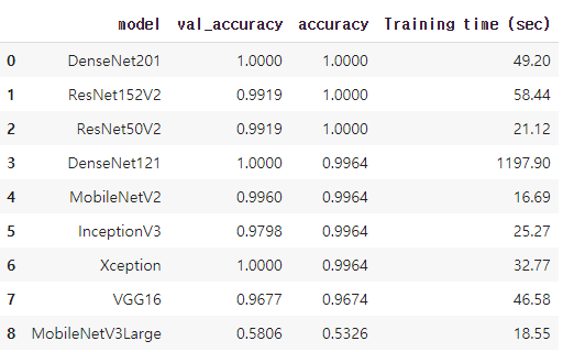
학습한 모델에 test셋을 통해서 전이모델별 성능을 확인했는데 정확도가 대부분 1에 수렴하는 것을 볼 수 있다.
plt.figure(figsize = (15,5))
sns.barplot(x = 'model', y = 'accuracy', data = df_results)
plt.title('Accuracy on the test set (after 1 epoch))', fontsize = 15)
plt.ylim(0,1)
plt.xticks(rotation=90)
plt.show()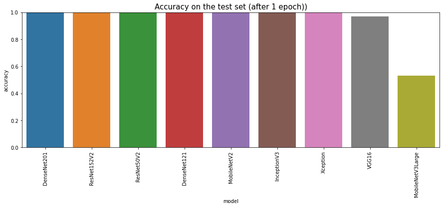
정확도를 시각화해보았는데 상위 7개 정도는 1에 가까운 값이 나왔다.
plt.figure(figsize = (15,5))
sns.barplot(x = 'model', y = 'Training time (sec)', data = df_results)
plt.title('Training time for each model in sec', fontsize = 15)
# plt.ylim(0,20)
plt.xticks(rotation=90)
plt.show()
모델 성능 확인 _ DenseNet201, ResNet152v2
VGG19모델처럼 시간만 오래걸리고 성능은 좋지못한 모델이 있기 때문에 가장 좋은 성능을 내고 시간도 적게 드는 Densenet201과 resnet152v2를 통해서 다시 성능을 확인해보았다.
좋은 효율을 내는 모델 성능확인 1 (DenseNet201)
train_df,test_df = train_test_split(df, test_size=0.1, random_state=0)
train_generator,test_generator,train_images,val_images,test_images=create_gen()

model = get_model(tf.keras.applications.DenseNet201)
history = model.fit(train_images,validation_data=val_images,epochs=7)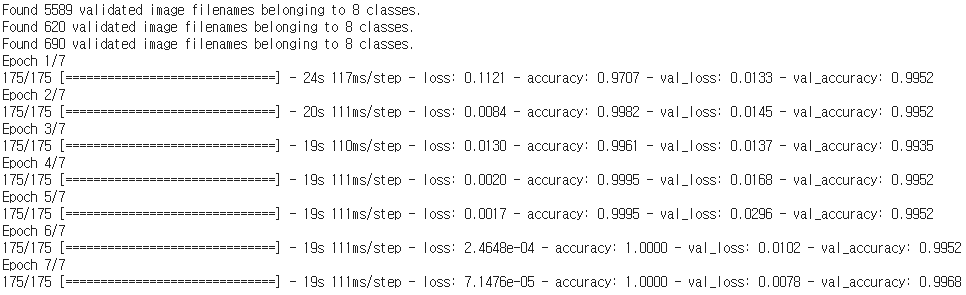
pd.DataFrame(history.history)[['accuracy','val_accuracy']].plot()
plt.title("Accuracy")
plt.show()
pd.DataFrame(history.history)[['loss','val_loss']].plot()
plt.title("Loss")
plt.show()
# Predict the label of the test_images
pred = model.predict(test_images)
pred = np.argmax(pred,axis=1)

# Map the label
labels = (train_images.class_indices)
labels = dict((v,k) for k,v in labels.items())
pred = [labels[k] for k in pred]

y_test = list(test_df.Label)
acc = accuracy_score(y_test,pred)
print(f'Accuracy on the test set: {acc * 100:.2f}%')
Accuracy on the test set: 99.71%
test데이터를 통해서 성능을 확인하니 Densenet모델은 99.71%의 예측률을 나타내었다.
좋은 효율을 내는 모델 성능확인 2 (ResNet152V2)
다음으로는 resnet모델을 학습했습니다. 5에포크로 학습을 진행했고 2에포크에서 정확도는 1을 로스는 0에 수렴했다.
train_df,test_df = train_test_split(df, test_size=0.1, random_state=0)
train_generator,test_generator,train_images,val_images,test_images=create_gen()

model = get_model(tf.keras.applications.ResNet152V2)
history = model.fit(train_images,validation_data=val_images,epochs=5)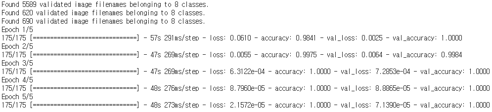
pd.DataFrame(history.history)[['accuracy','val_accuracy']].plot()
plt.title("Accuracy")
plt.show()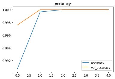
pd.DataFrame(history.history)[['loss','val_loss']].plot()
plt.title("Loss")
plt.show()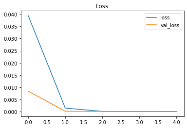
# Predict the label of the test_images
pred = model.predict(test_images)
pred = np.argmax(pred,axis=1)

# Map the label
labels = (train_images.class_indices)
labels = dict((v,k) for k,v in labels.items())
pred = [labels[k] for k in pred]

def printmd(string):
    # Print with Markdowns
    display(Markdown(string))

y_test = list(test_df.Label)
acc = accuracy_score(y_test,pred)
printmd(f'# Accuracy on the test set: {acc * 100:.2f}%')
Accuracy on the test set: 100.00%
마크다운언어로 출력하는 함수를 사용해서 좀 크게 보이게 설정하고 확인해보니 모델의 예측률은 100%의 성능을 나타냈다. 그래서 저의 목표인 100%의 성능을 나타내는 모델을 만드는데 성공했다.
성능 100% 모델의 정밀도와 재현율
이 모델의 정밀도와 재현율을 확인해보면 모든 라벨에 대해서 정확도 100%를 나타낸다.
class_report = classification_report(y_test, pred, zero_division=1)
print(class_report)
Confusion Matrix 시각화
Confusion 매트릭스도 히트맵을 통해서 나타내 보았는데 본인외에 전부 어두운색으로 나타낸다.
from sklearn.metrics import confusion_matrix
import seaborn as sns

cf_matrix = confusion_matrix(y_test, pred, normalize='true')
plt.figure(figsize = (10,7))
sns.heatmap(cf_matrix, annot=False, xticklabels = sorted(set(y_test)), yticklabels = sorted(set(y_test)),cbar=False)
plt.title('Normalized Confusion Matrix', fontsize = 23)
plt.xticks(fontsize=15)
plt.yticks(fontsize=15)
plt.show()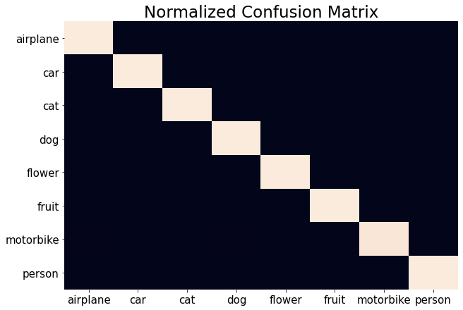
실전 : 모델 예측
모델을 실제로 확인해보기위해서 사진을 뽑아보고 그 사진에 대한 예측을 잘하는지 확인해보기
# from PIL import Image
import pandas as pd
from tensorflow.keras.preprocessing import image
import matplotlib.pyplot as plt
from tensorflow.keras.applications.inception_resnet_v2 import InceptionResNetV2, preprocess_input
def printmd(string):
    # Print with Markdowns
    display(Markdown(string))
class_dictionary = {'airplane': 0,
                    'car': 1,
                    'cat': 2,
                    'dog': 3,
                    'flower': 4,
                    'fruit': 5,
                    'motorbike': 6,
                    'person': 7}
IMAGE_SIZE    = (224, 224)
number_1 = int(input("번호를 입력하세요 : ")) # 10, 50, 100
test_image = image.load_img(test_df.iloc[number_1, 0]
                            ,target_size =IMAGE_SIZE )
test_image = image.img_to_array(test_image)
plt.imshow(test_image/255.);

test_image = test_image.reshape((1, test_image.shape[0], test_image.shape[1], test_image.shape[2]))
test_image = preprocess_input(test_image)
prediction = model.predict(test_image)

df = pd.DataFrame({'pred':prediction[0]})
df = df.sort_values(by='pred', ascending=False, na_position='first')
printmd(f"## 예측률 : {(df.iloc[0]['pred'])* 100:.2f}%")

for x in class_dictionary:
  if class_dictionary[x] == (df[df == df.iloc[0]].index[0]):
    printmd(f"### Class prediction = {x}")
    break
번호를 입력하면 번호에 대한 이미지가 나오고 그 이미지에 대해서 예측 라벨을 출력하는데 위의 결과를 보면 예측률 100%로 person을 잘 예측하는것을 볼 수 있다.
- 여러 이미지 예측
# Display picture of the dataset with their labels
fig, axes = plt.subplots(nrows=4, ncols=6, figsize=(20, 12),
                        subplot_kw={'xticks': [], 'yticks': []})

for i, ax in enumerate(axes.flat):
    ax.imshow(plt.imread(test_df.Filepath.iloc[i]))
    ax.set_title(f"True: {test_df.Label.iloc[i].split('_')[0]}\nPredicted: {pred[i].split('_')[0]}", fontsize = 15)
plt.tight_layout()
plt.show()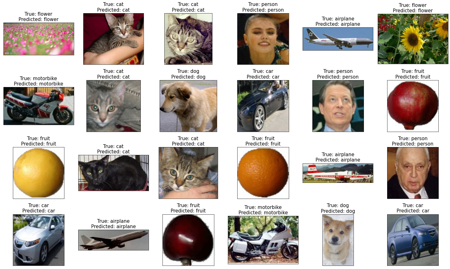
8개의 범주로 분류되어있는 10000개가 넘는 이미지 데이터를 100%에 근접하는 확률로 예측하는 모델을 만드는데 성공
출처
- 캐글 데이터셋
'IT이야기' 카테고리의 다른 글
| 딥러닝대회_열화상 이미지 객체탐지 경진대회(입상) (0) | 2021.12.24 |
|---|---|
| (데이콘) ML _ Project : 구내식당 요일별 점심, 저녁 식수 인원 예측 (0) | 2021.07.25 |
| Project : 다음 분기에 어떤 게임을 설계해야 할까? (0) | 2021.06.13 |
| [라이트봇] light bot 3단계 3-1 ~ 3-6 정답 (0) | 2021.05.22 |
| [라이트봇] light bot 2단계 2-1 ~ 2-6 정답 (0) | 2021.05.22 |